NeurIPS 2026
TIDE: Asymmetric Neural Circuits for Stabilized Temporal Inhibitory-Excitatory Dynamics
- 1Luleå University of Technology
- 2Örebro University
- 3RISE Research Institutes of Sweden
TIDE
CTM
Scroll the figure sideways, or tap it to open it full size.
Abstract
Recent Continuous Thought Machine (CTM) architecture decouples internal computation from external inputs via neural dynamics, but relies on unconstrained multi-layer perceptrons for its recurrent computations. We propose to model neural dynamics using asymmetric Excitatory-Inhibitory (E-I) networks, which can be stabilized via principles from network theory, while obeying Dale's principle and can be expressed as energy-based systems optimized through a game-theoretic loss. Building on this perspective, we introduce Temporal Inhibitory-Excitatory Dynamic Engine (TIDE), a neuro-inspired architecture that computes internal representations through neural dynamics stabilized by incorporating the Wilson-Cowan dynamics and lateral inhibition. TIDE balances biological realism by, for instance, using Hierarchical Receptive Fields and enforcing Dale's principle to ensure a realistic 80 : 20 E-I balance ratio with an end-to-end trainable architecture. The aim of this paper is to introduce a new architecture that brings neuro-inspired learning and architectural principles to the forefront. We present proofs of convergence, stability, and complexity bounds, along with empirical ablation studies. Overall, TIDE achieves higher top-1 accuracy than CTM on the majority of the investigated datasets while requiring a smaller training budget. Furthermore, across varying training budgets, TIDE improves top-1 accuracy on ImageNet-C by an average of +1.65% to +6.42% under different perturbation severity levels.
Demo
Each clip follows one ImageNet validation image through the 50 internal steps. The top row is TIDE and the bottom row is CTM. From left to right: the input, the mean attention, the attention overlaid on the image, and the five most likely classes with the certainty at that step. Press play to start a clip.
Six of the twelve clips in the supplementary material, chosen to cover every outcome: two where only TIDE is correct at the last step, two where only CTM is, one where both are and one where neither is.
Method
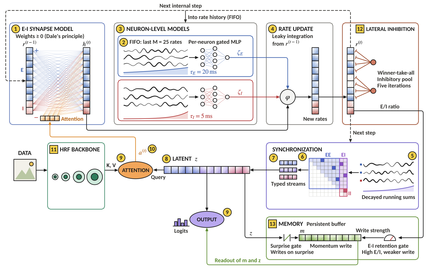
TIDE keeps the loop of the Continuous Thought Machine, a sequence of internal steps that is decoupled from the input, and changes what runs inside it. The neurons are split 80:20 into an excitatory and an inhibitory population. Every recurrent weight is non-negative, and whether a connection excites or inhibits is decided by the population it leaves, which is Dale's principle. The two populations follow a forward-Euler Wilson-Cowan update with their own time constants.
, , , and after every optimizer step.
Forward-Euler Wilson-Cowan update of the E-I rates. In TIDE, h is normalized by RMSNorm. The minus sign in front of the inhibitory term is explicit because the weights themselves are never negative.
From CTM to TIDE
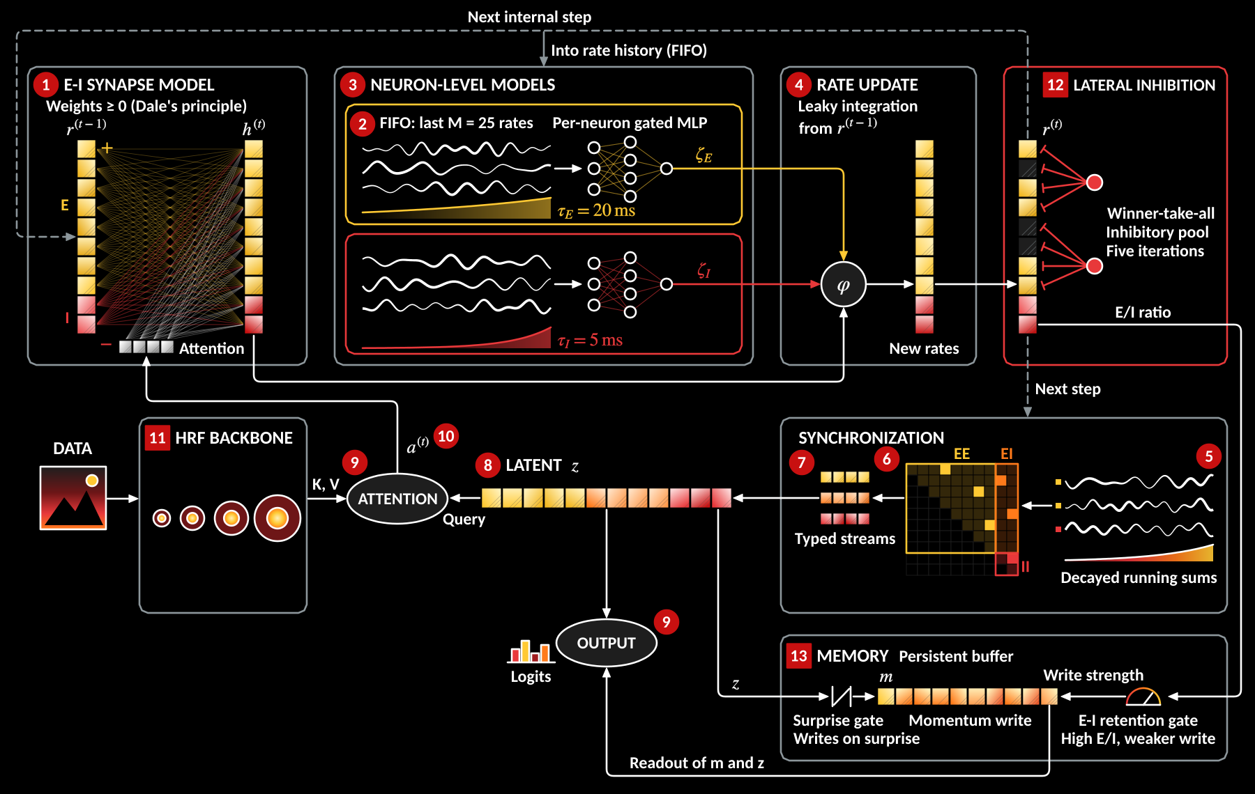
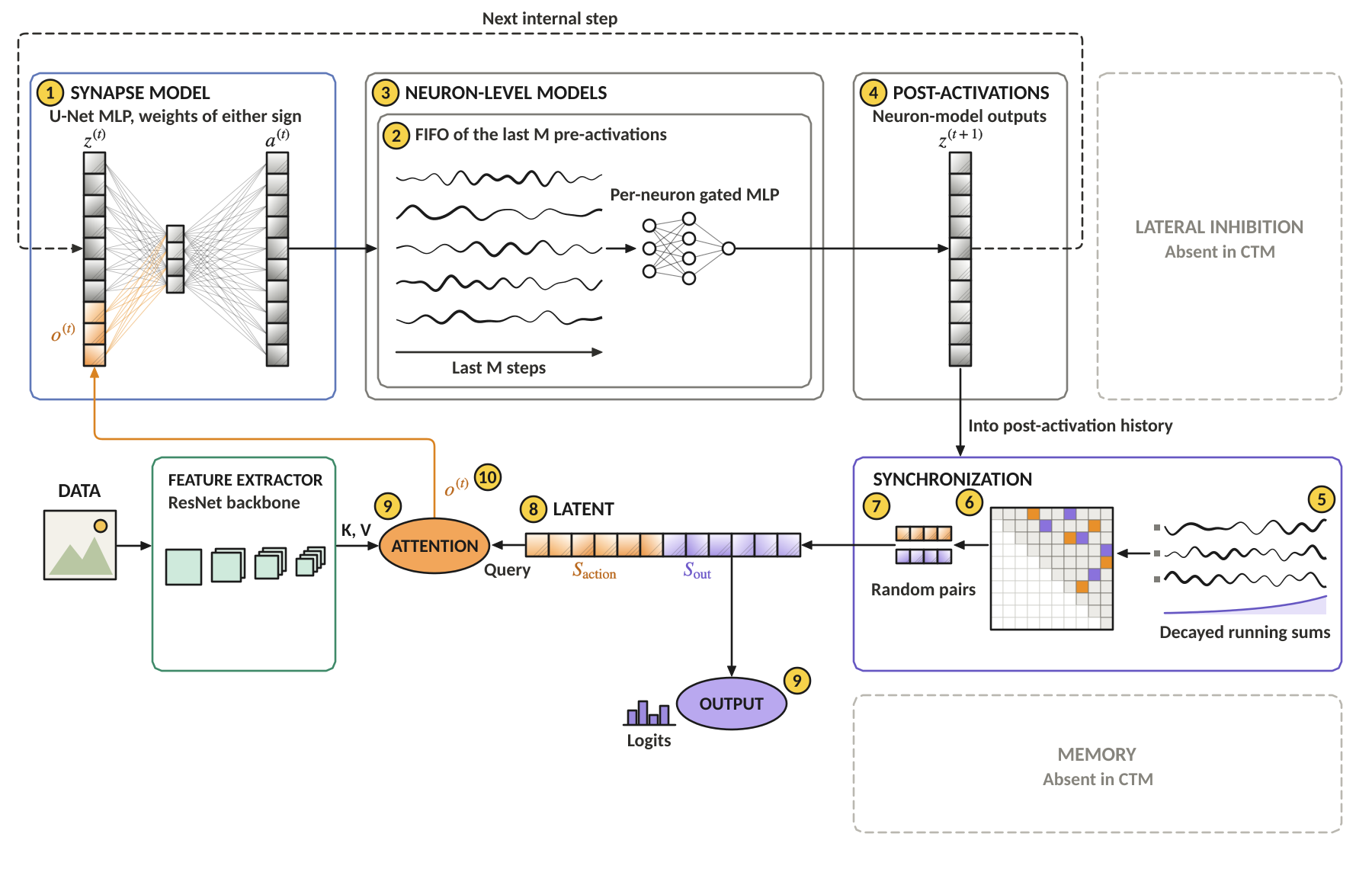
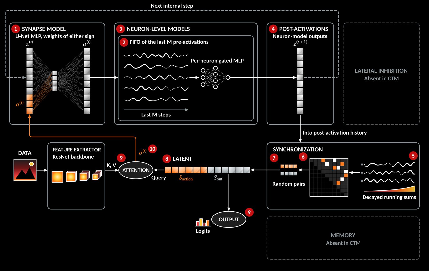
The figure at the top of the page shows both models on the same grid. The table lists the same changes block by block.
| Block | CTM | TIDE | Change |
|---|---|---|---|
| Feature extractor | ResNet backbone | Hierarchical receptive fields (HRF): learnable center-surround filters, trained end to end | Replaced |
| Neuron interaction | Synapse model: U-Net MLP with weights of either sign | E-I populations under Dale's law; all four weight blocks are non-negative and inhibition enters with an explicit sign | Replaced, split 80:20 |
| Neuron-level models | A single set of per-neuron models on the pre-activation history | Two sets on the rate history, one per population: τE = 20 ms and τI = 5 ms | Duplicated |
| Normalization | Shared LayerNorm | RMSNorm per population | Modified |
| Synchronization | Single stream | Three streams: E-E (binding), E-I (gating), I-I (rhythm) | Decomposed |
| Cross-attention | Query from synchronization | Adds a residual stream, a ← a + z, on ImageNet-1K | Added, conditional |
| Lateral inhibition | Absent | Winner-take-all on the excitatory population, five iterations | Added |
| Memory | Absent | Surprise-gated persistent buffer with momentum; an E-I retention gate weakens writes when the E/I activity ratio is high | Added |
| Output head | Reads the synchronization vector | Reads the latent and the memory, [z; m] | Extended |
What changes block by block, after Figure 1 of the paper.
Training and stability
- Training under Dale's principle
- Projected gradient descent: after every optimizer step the recurrent weights are clamped to W ≥ 0.
- Game-theoretic loss
- The E-I circuit is read as a game between neurons, and the loss penalizes the fixed-point residual of the per-neuron energies (Betteti et al., 2025).
- Stability
- Lyapunov diagonal stability is monitored during training through a differentiable Perron sum-ratio surrogate that caps ρ(WEE) and ρ(WII).
Results
TIDE and CTM are trained with the same seeds and the same number of optimizer steps on five image-classification datasets. CTM is retrained for this comparison.
| Dataset | Steps | dmodel | TIDE | CTM | ||
|---|---|---|---|---|---|---|
| mean ± std | best seed | mean ± std | best seed | |||
| MNIST | 50K | 256 | 99.64 ± 0.03 | 99.67 | 99.54 ± 0.03 | 99.56 |
| MNIST | 200K | 256 | 99.60 ± 0.05 | 99.64 | 99.59 ± 0.06 | 99.64 |
| Fashion-MNIST | 50K | 256 | 94.21 ± 0.21 | 94.42 | 92.51 ± 0.11 | 92.63 |
| Fashion-MNIST | 200K | 256 | 94.12 ± 0.19 | 94.23 | 92.53 ± 0.24 | 92.80 |
| CIFAR-10 | 600K | 512 | 90.62 ± 0.06 | 90.68 | 86.23 ± 0.34 | 86.59 |
| CIFAR-100 | 600K | 718 | 62.23 ± 0.16 | 62.38 | 65.19 ± 0.48 | 65.70 |
| CIFAR-100 | 600K‡ | 718 | 65.68 ± 0.18 | 65.79 | ||
| ImageNet-1K | 100K | 4096 | 67.22 ± 1.52 | 68.74 | 52.67 ± 1.79 | 54.46 |
| ImageNet-1K | 200K | 4096 | 68.40 ± 1.91 | 69.55 | 62.78 ± 1.31 | 64.06 |
| ImageNet-1K | 500K | 4096 | n/a | 69.90 | n/a | 71.78 |
Best top-1 accuracy (%) during training, as mean ± standard deviation over seeds and for the best seed (Table 1 of the paper). Bold marks the highest value per dataset and step budget, separately for the mean and for the best seed. ‡ Effective batch size of 64. At 500K steps on ImageNet-1K only one run per model is reported, and CTM attains the higher accuracy.
Component ablation
Each row removes one component from the full model, or adds the spectral regularizer, and retrains with the same seeds. MNIST and Fashion-MNIST use 50K steps, CIFAR-10 and CIFAR-100 use 600K.
| Configuration | MNIST | Fashion-MNIST | CIFAR-10 | CIFAR-100 |
|---|---|---|---|---|
| Reference | ||||
| CTM | 99.54 ± 0.03 | 92.51 ± 0.11 | 86.23 ± 0.34 | 65.19 ± 0.48 |
| TIDE, full (λspec = 0) | 99.64 ± 0.02 | 94.21 ± 0.21 | 90.62 ± 0.06 | 65.68 ± 0.18 |
| Component removed | ||||
| Wilson-Cowan update | 99.61 ± 0.02 | 93.70 ± 0.12 | 90.18 ± 0.26 | 64.52 ± 0.67 |
| Dale's law constraint | 99.59 ± 0.03 | 93.55 ± 0.18 | 89.01 ± 1.74 | 65.39 ± 0.39 |
| Lateral inhibition (WTA) | 99.61 ± 0.02 | 93.80 ± 0.17 | 89.13 ± 1.20 | 64.94 ± 0.30 |
| Surprise-gated memory | 99.59 ± 0.01 | 92.95 ± 0.16 | 88.97 ± 1.41 | 64.32 ± 0.30 |
| HRF backbone (ResNet-18 instead) | 99.60 ± 0.03 | 93.03 ± 0.12 | 83.02 ± 2.02 | 54.49 ± 0.76 |
| Component added | ||||
| Spectral regularizer (λspec = 0.1) | 99.64 ± 0.03 | 94.31 ± 0.06 | 89.02 ± 2.93 | 65.38 ± 0.35 |
Leave-one-out ablation: best top-1 accuracy (%) during training, mean ± standard deviation over seeds (Table 3 of the paper). Bold marks the highest value per dataset. Removing the memory costs the most on MNIST and Fashion-MNIST; swapping the HRF backbone for ResNet-18 costs the most on CIFAR-10 and CIFAR-100.
Attention over internal steps
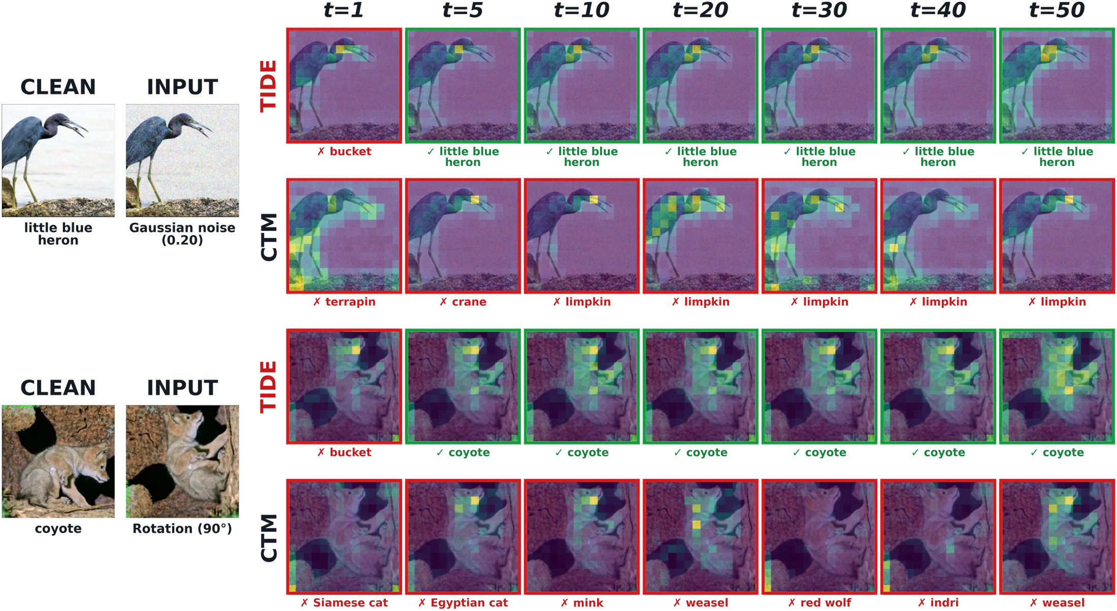
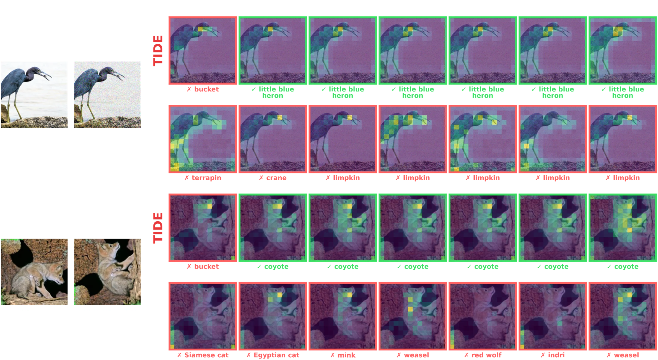
Scroll the figure sideways, or tap it to open it full size.
Robustness
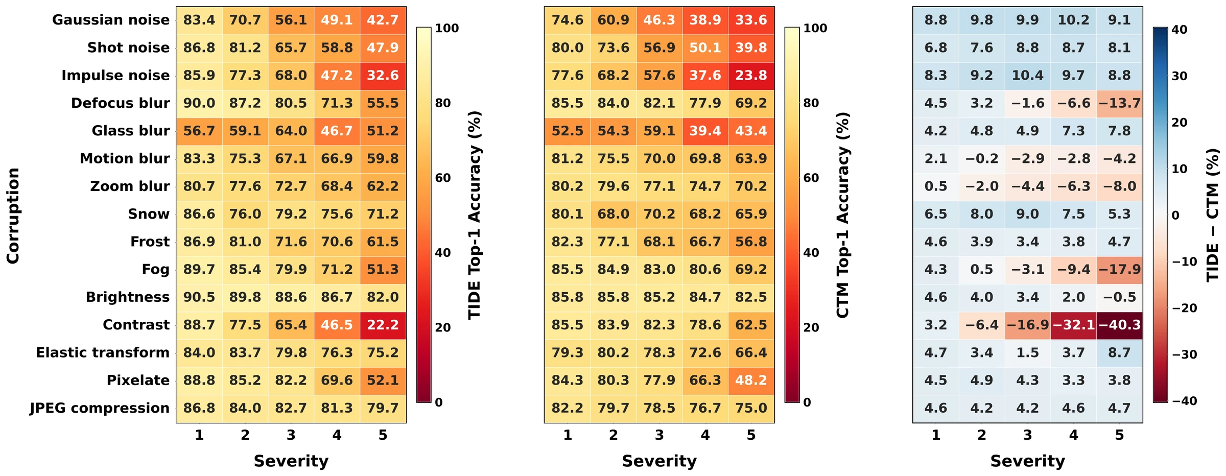
Both models are trained on clean ImageNet-1K only and then evaluated on ImageNet-C, which applies 19 corruption types at five severities. At 500K training steps TIDE is ahead of CTM by 2.68 points on average over all 95 cells. With smaller training budgets the gap is wider: 16.8 points at 100K steps and 6.4 points at 200K. CTM is the more robust of the two under fog, frost and snow.
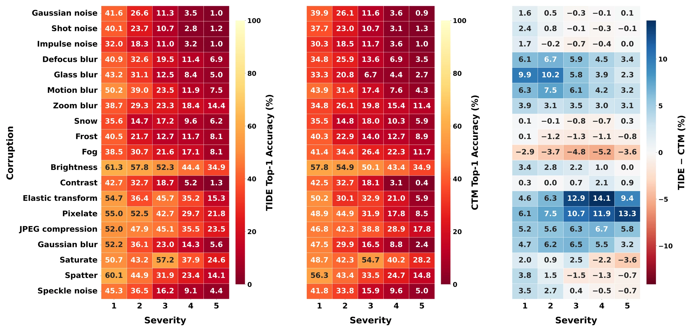
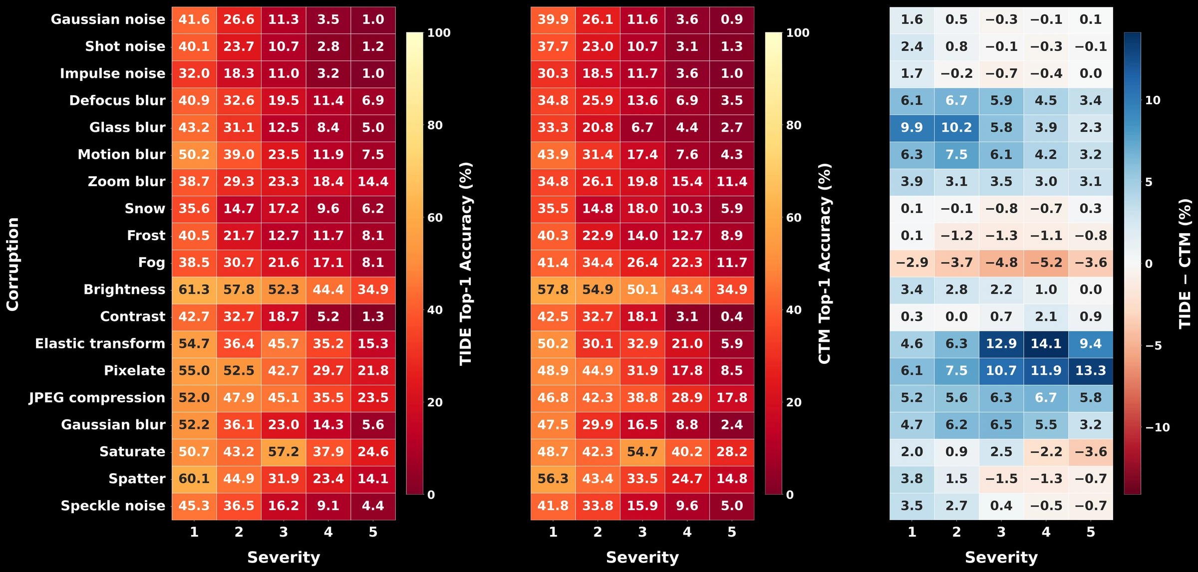
Scroll the figure sideways, or tap it to open it full size.
On CIFAR-10-C the results are mixed. TIDE leads under noise and under snow and frost, while CTM is clearly better at high severity under contrast, fog and defocus blur.
Scroll the figure sideways, or tap it to open it full size.
Limitations
The main limitation of both TIDE and CTM is their required sequential feedforward data processing, which prohibits shorter runtime and prevents more robust investigation. Therefore, further investigation is required to assess the feasibility of leveraging neuromorphic hardware and its dynamics, not only to enhance data preprocessing but also to implement a Look-up-Table-based approach to further reduce the training duration of the proposed framework. Given that we have already lowered the training boundary by around 50% to achieve results comparable to CTM, indicating the soundness of our approach, further studies are still needed to assess the reachability of an even sparser representation. Additionally, due to the lack of comparable implementations using similar approaches, detailed benchmarking within the same architectural family remains limited and challenging. Although CTM uses LSTM as its baseline, it is not a direct comparison; however, their results can be directly translated to TIDE given that we use CTM as our baseline.
The limitations paragraph of Appendix H of the paper, word for word.
Citation
@inproceedings{
anonymous2026tide,
title={{TIDE}: Asymmetric Neural Circuits for Stabilized Temporal Inhibitory-Excitatory Dynamics},
author={Anonymous},
booktitle={The Fortieth Annual Conference on Neural Information Processing Systems},
year={2026},
url={https://openreview.net/forum?id=dwcrK8NHpm}
}